
Simple Electron Microscopy Primer
Back projection is the process by which we generate our 3D model. As was discussed earlier, one of the goals of single particle analysis is to use 2D images formed by TEM to reconstruct a 3D model of the original object. In this section, we will see how the generated projections are "added up" to recreate the model.


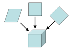
As its name implies, back projection is the inverse function of projection. When an n-dimensional object is projected, each projection is an n-1 dimensional sum of its density along the projection axis. Therefore, a sphere would have circles as its projections. A cube, on the other hand, would produce either squares, diamonds, or other intermediate parallelograms (Figure 1 top) depending on the direction of projection. The actual shape, of course, depends on the orientation from which the projection was made. The reverse function (Figure 1 bottom) is called back projection and regenerates the original object.

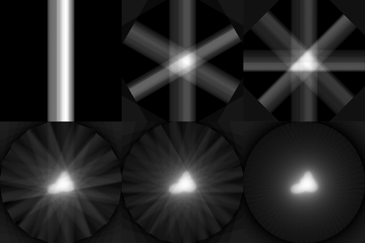
Since a projection can be thought of as a "squishing" of the object, back projection is then the "smearing" of the projections back onto each other. The sum of the back projected projections regenerates the original object. In the example above, a cube generated different paralleograms in projection. In Figure 2, back projected circles were used to reconstruct the original sphere. When a circle is "smeared" along its axis towards the center of the space, it forms a line. In each frame of the animation in Figure 2, more of these back projected lines are added at different angles. As the amount of projections used is increased, the lines complement each other where they intersect. The result is that the sphere at the intersect point becomes better defined. Thus, the back projection of the projections can reconstruct the original object.
The following example presents a more detailed view of back projection using a more complicated model with extra features and details.


The Radon transform is an algorithm that transforms an original image into a series of equiangular projections. When applied to a 2D object, the output of the Radon transform is a series of 1D lines. For easier representation, the lines are often stacked on top of each other, generating a sinogram. The sinogram in Figure 4 is the Radon transform of Figure 3.

To create the different figures for this example, the following SPIDER script was used: b00.radon.spi. This script generates a Radon transform from the input model, extracts each individual projection from the sinogram, and modifies the projections so that they can be averaged. While the script is not a mathematically accurate description of back projection, conceptually it is similar. Finally, it can be easily modified for other presentational examples.
The above descriptions dealt with an ideal sample. All the information from the original model was known. This made it easy for the reconstruction programs to recreate the original model with high fidelity. But what happens with a real world example? Data is often missing or inaccessible.
In the previous steps of the reconstruction process, the experimental particles were centered and aligned. Lastly, each experimental projection was assigned a set of Euler angles that define its position in space relative to its origin from the original model.

To generate Figure 5 all the projections were evenly spaced around the origin. All of Euler space was covered. In a real world example, the experimental projections are usually either randomly distributed or heavily biased and clustered towards one orientation. Ideally, an even, random distribution is prefered. However, this is rarely the case. When experimental projections are clustered, some views will be over represented over others. This results in a skewed final reconstruction. Figure 6 is such an example of a biased reconstruction. The original model is the same as in Figure 3, but the back projection was only limited to half the projection data set.